On learning Calculus

I started this journey with a the following concern: would I be able to learn Calculus, or is it something beyond my reach?

I think I have answered that question this year. I am quite able to learn Calculus and I have actually learned some. My statement of intent was "to learn and master Calculus", which now sounds like a very bold statement. I believe I would have needed many more years to master a discipline as vast as Calculus. However, my new understanding of it fills me with satisfaction. I have indeed attained closure on a topic that was as personal as it was academic.

What do I take with me? Quite a lot actually, from the importance of starting with a good base, to the realization that I learn best with the structure of a course than on my own. I also take limits both as a mathematical concept as well as life concept. One helps you explore infinity, the other, I realized, is mainly in your mind. I take differentiation and integration, since at times is important to know the guiding essence of a thing and at others the power of togetherness.

I also learned a lot about change.

Change of rates as well as change of heart. Change as the definition of what we are and were we are going.

I am happy I did this project. It has been hard, it took a lot of time and effort. I made some hard sacrifices as time. But I made it.

I want to thank my wife María del Carmen for her love and support, and also my daughter Amanda for putting up with me calculating away some Saturday mornings. I could not have done it without you. You are, ahem, integral to me. I love you.

So here it is, the end of this blog, I guess. The last entry. Thank you Calculus, it has been a blast.

 

The fundamental theorem of Calculus

Here I am. At the end of my project. My next to last post. And my topic is the fundamental theorem of Calculus. Like the name says, this theorem is a pretty big deal. Let's start by what the Theorem says according to Wolfram Alpha:

I can proudly say I actually understood some of that, but at first could not yet grasp the implications that statement had on all I had studied so far.

Here is Dr. Fowler from Mooculus.com explaining this theorem and it's implications brilliantly:

Now here is what (I think) the fundamental theorem of calculus means in my own words. If you want to integrate acontinuous function on a closed interval, instead of doing the limits of the Riemman Sum applicable, just find the anti-derivative of the function you need to integrate and substract the result of the evaluation of that anti-derivative at the befining and end points of your closed interval.

Or in better words, forget about integrating, just anti-diferentiate!

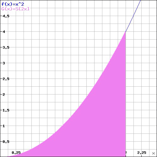
In my last two posts I had been searching for the area under the curve of x² from the interval 0 to 2. And I had to do a bunch of sigma calculations and set up Riemman Sums and then even take a limit in order to get to 2.667 square units which is 8/3.

The fundamental theorem of calculus is, as I see it, a reward for all my efforts. It is a way of saying:"Fernando, you have toiled and fret, and sweated over these sums and spend countless pages calculating and recalculating all these stuff. You have earned a shortcut." Why thank you very much calculus!

Do you want to check out my new super power? Ok.

The FTOC is telling me that to integrate from the interval a=0 to b=2 of the function x² all I need is an anti-derivative of that formula which I will proceed to evaluate at both points of my interval and then subtract. What is an antiderivative of x²?

Technically there is a + C after that formula but I am assuming it is 0, check Dr. Fowler's video again for that to make sense.

Ok, so now I have my antiderivative x³/₃ and I am ready to evaluate it at 2 (b=2) and at 0 (a=0) and then take the difference .

Now let's plug it back into the formula for the fundamental theorem of calculus.

And finally we get:

There you have it, the elusive 2.667, the area under the curve of x² From the interval starting at 0 ending at 2.

Wow, that took way less effort than before. However, If I had not passed through all those previous steps, all that trouble and effort, I would not have appreciated the beauty, simplicity and deeper meaning of what I have accomplished.

This is my next to last post in this blog and it is a fitting one. I cannot begin to express the emotions I feel at the moment. I have attained great insights in this journey. I now have a deeper understanding of math and the world around me.

Let me know your thoughts in the comments section.

 

On integrating and finally integrating

I wish I could explain how satisfying it is to finally learn the concepts of integration in calculus. For years I have seen how people would represent calculus with a picture of a curved function with the area under it shaded, and for the life of me, I could not figure out how they would calculate that. Now I know. The relative simplicity of the process has a ring of truth, and symmetry, and beauty that threw me back to discovering geometrical theorems in high school.

Well, here it goes: Integrals as I understood them.

Imagine you have a formula that is continuous at least for a given interval [a,b]. I chose again x² in the closed interval form 1 to 2. I already tried to find the area under that curve in my post on Sigma.

By using 10 rectangles of width 1/5 and height x², I was able to approximate the area under the curve to be 2.28 square units an underestimation of the true area. However, I posted that I could get better approximations if my rectangles had been infinitely small.

To get those better approximations I need to improve the sum I used before, pictured to the right. And in order to do that, I would need to convert it into a Riemman Sum.

The toughest part of doing integration is to set up the correct Riemman Sum for the purposes intended. I struggled so hard with this part that I want to give you this video to follow just in case I mess up. Here is the general formula for a Riemman Sum:

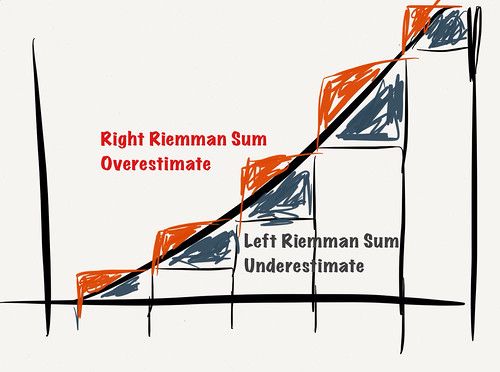
Since I am doing a right Riemman Sum, I will use this version of the formula. Where a and b are the interval of my function, and n represents the times I will be cutting that interview. A right Riemman sum will give me an overestimate of the area under the curve, which will complement the underestimate of 2.28 I got

 

The first thing you need to do to set up a Riemman sum is deciding what your interval is (in this case is from 0 to 2) and then decide how wide you want your divisions within that interval to be. I want my intervals to be 1/5 units wide, but that is not important right now, just remember there are ten 1/5 divisions from the interval 0 to 2. Then for the height of my rectangles I chose to evaluate the function x² on the right hand side of those intervals. With those steps selected then I follow the x² rules for Riemman Sums.

A Riemman Sum is the addition of the formula I want to evaluate (x²) at the specific cuts I made. The first point on my interval is a=0 and the last point is b=2. I want to divide that interval in n cuts of a certain size. The formula for the cut size is:

Now here is the formula for the height of my rectangles.

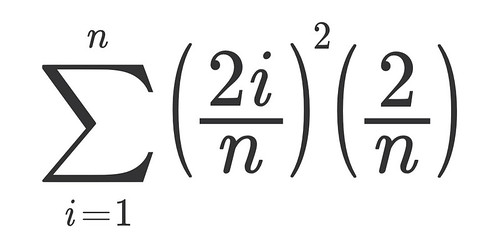
So putting all the steps together here is the formula for my Riemman Sum

And that is actually the hard part, for me at least. The rest is arithmetic.

So the answer I got was: 8/3 + 4/n + 4/3n²

But what does that mean? Remember when I said I wanted the width of my rectangles to be 1/5 units and that it meant I would get 10 segments from interval 0 to 2? Well, if you substitute n=10. The area under the curve it gives me is 3.08 square units.

Now since this is a right Riemman sum I know it is an overestimate. My last attempt in the Sigma post was equivalent to a left Riemman sum which gave me an underestimate of 2.28.

If I take the average of these two numbers I should be able to get a better estimate of the area under the curve: (3.08 + 2.28)/2 = 2.68.

And 2.68 is very close to the true area under the curve which is approximately 2.667. Now, how can we get there?

Well supposed that instead of splitting my interval of this Riemman sum into 10 pieces I split it into 100, n=100, what happens then? We get 2.708 instead of 3.08. And what if n=10,000, that would make our rectangles very, very small, we then get 2.670! That is very, very close to 2.667

And what if n=infinity?

Then the n in this formula 8/3 + 4/n + 4/3n² would be so small (and therefore the width of the rectangles would be also so small) that the only effect relevant in 8/3, and guess what 8/3 comes down to: 2.667 approximately.

 

And what did we just do? We just took a limit.

Whoah! What?!!

Yes, we took the limit of our formula to get the true area under the curve. And that my friends is called integration.

To integrate is to do the following:

To take the limit of the Riemman Sum you are working on as n approaches infinity.

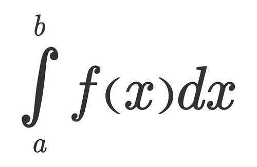
In fact the definite integral is a normally written as a variation of the formula above.

The elongated S just means, take the limit of the sum of f(x) times the change of x from the interval from a to be, as that change of x gets infinetly small.

And there you have it. Integration via the sum of infinite rectangles.

This one was a tough one and there are some considerations to this integrations stuff, but you can review them here.

Let me know what you think in the comments.

 

Area under the curve: Sums and Going Sigma

At last I reached the integral part of Calculus. I was eager to get there since it dealt with a topic which I find fascinating, how can I find the area of a curved object.

You see, area for me,and for the rest of the world, is width x height. Which is pretty simple if you are dealing with rectangles. However, what happens when you are not dealing with straight lines and need the area of a curved region. Well, apparently you just part from what you know and build a bridge!

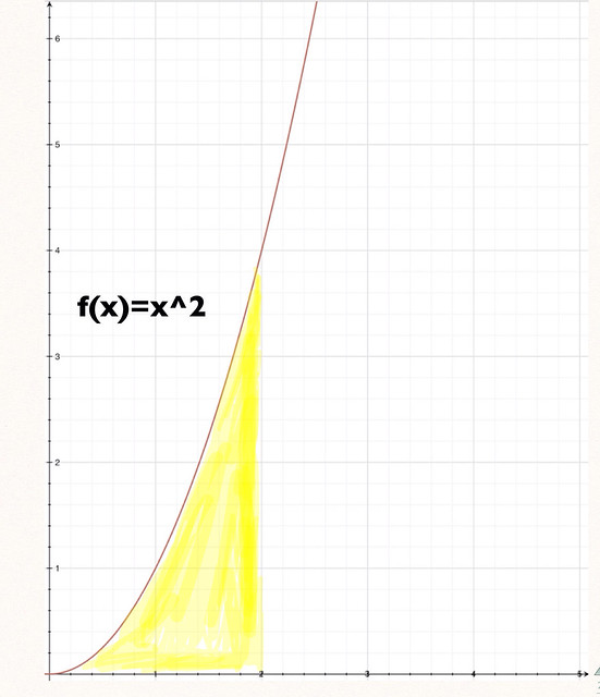
What I mean by that is that if I wanted to find the area under a curve like the one in the picture opposite. I can draw rectangles under the curved region up to the function and approximate it's area by summing the areas of all the rectangles I drew. That is a neat trick that has served humanity for centuries. And the cool part is that if I can make the rectangles thin enough, I can get a better approximation of the area I am looking for.

If the concept of getting better approximations by making an interval smaller and smaller a sounds familiar it's because we saw it back in limits and derivatives.

So how do I go about summing all these rectangles? I mean of they are 5 or 10 it's simple enough to do it by hand, but what is they are 100 or a 1000...or n rectangles!

That is were sigma comes in.

Have you met sigma? That weird looking capital E that might hunt your math nightmares. It turns out it is tame enough once you get to know it.

 

Sigma is just notation for adding something over and over again. I loved it when Professor Fowler at Mooculus compared it to using a "loop" in programming. It basically encodes and bounds a sum for a specified interval. One of the things I remembered having problems with was the notation used in sigma. For some reason back in college I found it difficult and unapproachable. Now it looks quite simple.

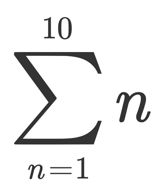
Let's imagine I want to add 1+2+3+4+5+6+7+8+9+10. If I have to write that sum over and over again it gets kinda tiresome. So I will use sigma as shorthand for that sum. But first, let's think about what I am summing: the number (whole numbers; integers; in order) form 1 to 10. So if I had a machine that would spit out a one then a plus sign then the next number after one and so on, I would replicate that string of numbers above. Well that is what sigma does, let's see:

Whenever you see that weird E, just imagine it is saying "please add the result of whatever formula is after me, starting with the number that is under me in the variable and repeating the process as many times as the number above me while making n to be a whole number greater after every repetition." Well, at least it said please.

Okay, first we have that n is the formula we are summing. Then under Sigma is an n=1, meaning the first result is 1. The it is asking us to repeat the process 10 times, that is the number over sigma. However, after each repetition we must make n a number greater than before.

So we start with n=1, then add n=2, then add n=3 and so on until we add n=10, 1+2+3+4+5+6+7+8+9+10! For a better (much better) explanation you can go here.

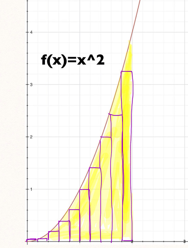
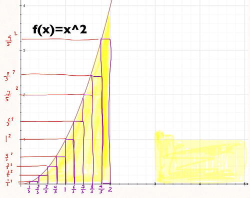
So if I take the example above, and lets say I divide the area under the curve into 10 sections of 1/5 square units, whose height is the formula f(x)=x² evaluated at those cut points.

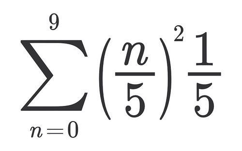
Therefore, the first rectangle would have area 0² times1/5=0, the next would have area (1/5)² times 1/5=.008, the one after would be (2/5)² times 1/5=.032 and so on. We could represent that sum this way, at least I think we could:

I Sigmalize we are saying square the 5th of whatever n is from 0 to 9 (the height of our rectangles), then multiply it by 1/5 ( their width) and Sum all 10 results.

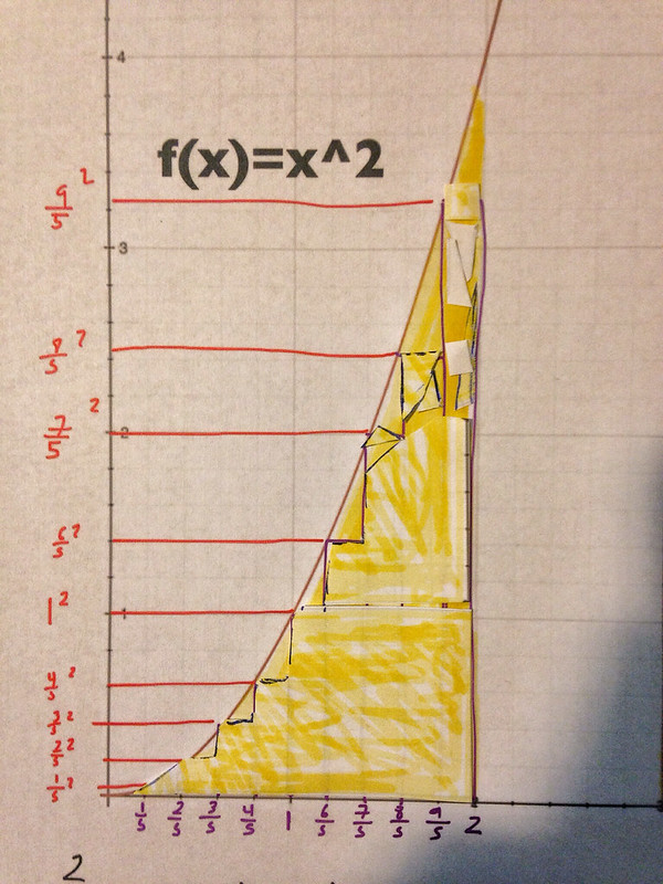
This will give you an answer that the area under the curve is approximately 2.28 square units.

That is not bad as approximations go. If you see the two pictures bellow, I shaded the 2.28 square units and pasted them to cover my rectangles.

But as you can see, I could not cover all the area under the curve. There are some triangles that go from the base of the rectangles up to the curve that I cold not cover. To cover all the area under the curve I would need to make smaller and smaller rectangles. In fact if I could make those rectangles infinetly small, I could approximate almos exactly the area under the curve.

I'll give you a preview. The area under the curve is actually closer to 2.666, but we will need to use something I have been looking forward to learning for a long time: Integrals.

Let me know if I got this right in the comments.